Tableau - Relationships : How LoD Works

In Tableau’s new data model, a logical layer is introduced over the physical layer. Tables on the logical layer are called logical tables, which are related to each other through the fields specified on the canvas. The physical layer is what the model used to be, where we can join and union tables. A very critical concept we would like to place emphasis on is that relationships don’t join all logical tables together as one merged table, indeed, they are like contracts describing how tables are related to each other. The timing for joining tables is upon analysis, namely, creating a viz. At that time, the join type will be determined based on the dimensions and measures used in the viz, and only the relevant data will be queried from the relevant tables. When click on View Data button on Data panel, we can see data records from each independent table but can’t see the combined records across all tables. 

As Tableau Help states, “Relationships are a dynamic, flexible way to combine data from multiple tables for analysis.”

As to relationships, the references listed on the bottom of this blog give a complete view. So, we won’t try to cover all the details here, on the contrary, we will look into several typical scenarios and see how relationships work, especially from the perspective of level of detail.

The model stated below will be used for the demonstration. TblSubA and TblSubB, joining on physical layer, form TblMain that acts as the main logical table. TblMain is related to TblHigher and TblSame and TblLower that have a higher, same and lower granularity against TblMain, respectively.

Data Model

 

Physical Layer 

Relationship between TblMain and TblHigher

 

Relationship between TblMain and TblLower 

Relationship between TblMain and TblSame

Sample records from each table are shown below.

Each table contains a measure.
Each table contains at least one record unmatched with the related table. 

TblMain has a granularity of Region – Branch – Employee.

 

Data Sample in TblMain

 TblHigher’s granularity is at Region level. One note, Constant field is not used in this post.

Data Sample in TblHigher 

TblSame take the same granularity as TblMain.

Data Sample in TblSame 

TblLower goes down to Product Category level compared with TblMain. It has a granularity of Region – Branch – Employee – Product Category. 

Data Sample in TblLower

 

Scenario : TblMain – TblHigher

First, we take a look at a classical case, calculating the ratio of (Sum of Sales / Sum of Goal) per region, which is previously solved by LOD expression or data blending. The LoD of the view is defined by Region which we get from TblHigher. Goal measure comes from the same table as Region dimension. Sales measure is taken from more granular table TblMain (Region – Branch – Employee).

Sum of Sales per region is correctly computed. So is Sum of Goal, as the following viz indicates. 

Then we add Sum of Sales / Sum of Goal to Marks, as a result, we get the exact ratio as expected. It is quite straightforward. And more, this data source can be published as one to Tableau server. 

Here is the summary data used in the view. 

Let’s do one more test, adding Branch from TblMain to the view. View’s LoD goes down to Region – Branch. This causes that Goal is duplicated as many as number of branches in a region, as illustrated in the screenshot below.

 

Scenario : TblMain – TblSame

When the tables have the same granularity, any LoD of view won’t produce duplicate data. For example, we would like to discover whether there is any correlation between Sales and Discount.

We bring Employee ID into the view. So, the view shares the same LoD with the data source which is made of TblMain and TblSame in this case.

Let’s try to roll the LoD up to Region. It works perfectly without any surprise. 

Since TblMain contains a record not matched in TblSame, and vice versa. It is a good example for us to explore more about how this is handled.

We drag and drop a dimension and a measure from TblMain to the view. This simply queries data from only TblMain, as we can see, there are no null values in the view. 

 Then, we add a measure from TblSame into the view, let’s see what will change.

Drag and drop Discount on Detail box in Marks. Obviously, a null value is included in the view. The underlying data also says so.

 If we add a dimension instead of a measure from TblSame to the view, will this make a difference? Yes, we won’t see a null value popping up on the view.

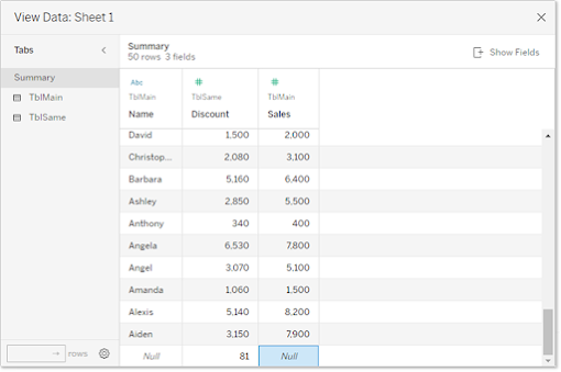
XnoneA is not findable in TblSame, so its Name(TblSame) is null; however, this won’t affect how the view presents.

For null values, we can use measure filter to filter them out.

Scenario : TblMain – TblLower

The pair works as similarly as TblMain – TblHigher does. When the LoD of view is kept not lower than TblMain’s, everything works well. Of course, null values show up in the view. But this is expected since we have measures from both tables in the view. 

LoD of View: Region

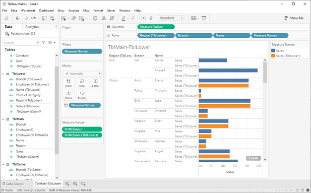
LoD of View: Region- Branch - Employee

What if we bring Product Category dimension to the view? LoD of view is less than that of TblMain. This leads to duplicated Sales (from TblMain), as the screenshot shows.

LoD of View: Region – Branch – Employee – Product Category

Scenario : TblMain – TblHigher – TblLower

This is multiple tables related scenario. In effect, we can imagine how they work based on the results of the above scenarios. So, we would like to test some cross-table calculations including LoD expressions here.

First, we look at the numbers at regional level, and we use text table for illustration this time. The measures are listed up as follows.

Goal from TblHigher (LoD: Region)

Sales from TblMain (LoD: Region – Branch – Employee)

Sales (TblLower) from TblLower (LoD: Region – Branch – Employee – Product Category) 

And, we also include a cross-table calculation into the view.

CompleteRatio = SUM([Sales]) / SUM([Goal]) 

The text table gives us the result exactly as expected. 

Subsequently, we start to add more dimensions to the view, in other words, lowering LoD. Let’s see what is going to happen. 

We add Branch (TblLower) to Rows shelf, as a subsequence, Goal is duplicated as Totals in chart tell because Goal comes from TblHigher.

Now, we create a new LoD calculation named by RegionalGoal and add it to the text table.

RegionalGoal = {FIXED [Region]:SUM([Goal])} / {FIXED [Region]:COUNT([Branch])} 

Total of column shows it removes the duplicates.

What if we add the following calculation to the view? 

RegionalGoal (TblLower) =

{FIXED [Region (TblLower)]:SUM([Goal])} / {FIXED [Region (TblLower)]:COUNT([Branch (TblLower)])}

 It gives a different result from RegionalGoal. 

What does cause the difference? Let’s examine the underlying data.

Divisors, {FIXED [Region]:SUM([Goal])} and {FIXED [Region (TblLower)]:SUM([Goal])}, produce the same result.

Dividends, {FIXED [Region] : COUNT([Branch])} and {FIXED [Region (TblLower)] : COUNT([Branch (TblLower)])}, produce different counts, as we can see from the below screenshots.

As we go down to TblLower, the number of branches associated with region Chubu is exactly same as that on the screenshot.

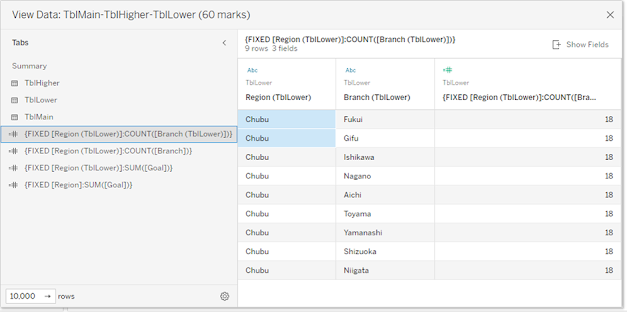
Noted LoD expressions behave differently against common calculations. Moreover, we can smell Order of Execution here. But we are not going to touch more in this blog.

For reference, if we modify the formula a little, using COUNTD in place of COUNT, it will give the same result as RegionalGoal. 

RegionalGoal (TblLower) =

{FIXED [Region (TblLower)]:SUM([Goal])} / {FIXED [Region (TblLower)]:COUNTD([Branch (TblLower)])}

 

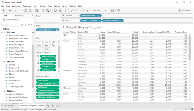
Let’s move back to the track and see how the view looks if we add Name (Employee) and Product Category from TblLower to the view. So the view has the same LoD as TblLower.

After we checked out the text table, measures from TblLower or having TblLower’s LoD are computed correctly, as Totals indicate.

Regarding cross-table calculations, here is an excerpt from Tableau Help, for reference.

“Be aware that cross-table calculations use inner join query semantics by default. The calculation lives on top of the join between the logical tables that it references. Also, it is now possible to write row-level calculations across tables that result in outer joins.”

Scenario – Constant

 Let’s create a calculation called ConstantOne that is equal to 1 and add it to the view. The view simply shows 1 on the chart.

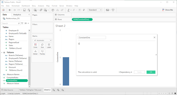
What about we drag and drop Branch from TblMain on Detail box in Marks? Sum of ConstantOne equals to the number of branches.

 Then, add Product Category from TblLower to the view. Sum of ConstantOne increases accordingly. 

So we can draw a conclusion, ConstantOne takes the LoD of dimensions in the view.

Relationships are used when combining data from different LoD, and support full outer joins As well. The related fields are fixed, not like Data Blending, we can assign key fields for each view. We can also adjust Cardinality and Referential Integrity settings on Data Source tab to optimize queries. After related necessary logical tables, we can publish them as one data source. But we can’t relate published data sources, and we can’t use calculated fields or geographic fields for defining relationships.

References:

 Relate Your Data – Tableau Help

Relationships, part 1: Introducing new data modeling in Tableau

Relationships, part 2: Tips and Tricks

Relationships, part 3: Asking questions across multiple related tables

Tableau - LOD Expressions

 

Before we dive into LOD expressions, namely, FIXED, INCLUDE and EXCLUDE, let's take a look at data source level of detail and view level of detail.  To make it clear, data source refers to the dataset appearing on Data pane on the left side of Tableau window, rather than the one in a database. It may be processed through Tableau Prep or Physical layer on the data model. Be noted, relationship in the new data model combines data from more than one tables in a dynamic and flexible way. To demonstrate the concept of LOD expressions in an easier manner, we will not discuss relationship here.

Simply put, data source has the finest granularity which can only be rolled up in the visualization. Data in a view is summarized by dimensions integrated into the view. As shown on the picture below, any dimension dropped into the red boxes will affect the granularity of data used in the view. They all together consist of the view level of detail. (Noted the super store dataset is employed for the demonstration.)

• Country
• Month Of Order Date
• Product Sub Category
• Ship Mode

Figure 1: View Level of Detail

You can right click on the view and select View Data menu to check the data set behind, as shown below. The measure value is summed up by the above dimensions.

Figure 2: Underlying Data

On the other hand, the original data source contains more dimensions, for example, City, Customer Segment, Product Category etc., as shown on the following figure. 

After we built a concept of data source level of detail and view level of detail, it becomes easier to understand LOD expressions. In nature they bring a summarized measure value with a different LOD into the view. 

FIXED

The expression is to calculate the measure by the dimensions designated in the formula. The calculation will not be affected by the view level of detail.

EXCLUDE

EXCLUDE expression will take the specified dimension away from the view level of detail while calculating the measure. 

Let's take a look at the example below. The view shows the quarterly sales for each product category. The view LOD is defined by Order Date (Quarterly) and Product Category. In case that we want to present the total sum of all product categories at the same time, let's see how EXCLUDE expression can help us achieve this.

Drag and drop Sales to Detail box in Marks card.

Replace the aggregation function with the following expression.

{EXCLUDE [Product Category] : SUM([Sales])}

Change it from Measure to Attribute using the context menu.

Add it to Tooltips as shown below.

As expected, we get the total amount of sales per quarter..

One note, EXCLUDE expression is not suitable for row-level calculations, as Tableau Desktop Help states.

"EXCLUDE level of detail expression cannot be used in row-level expressions (where there are

no dimensions to omit), but can be used to modify either a view level calculation or anything in

between (that is, you can use an EXCLUDE calculation to remove dimension from some other

level of detail expression)." - Create Level of Detail Expressions in Tableau Section, Tableau Desktop and Web Authoring Help

INCLUDE

INCLUDE expression will do the calculation by integrating the specified dimensions into the view level of detail. So it will further down the granularity of data in the view.

The below bar graph shows the total sales per quarter. If we would like to display the average sales per category on this chart, INCLUDE expression is a good option for this. On the second thought, I wouldn't see much business meaning to do so, considering the point is to demonstrate how INCLUDE expression works, so let's start with building the formula.

Create a calculated field named by SalesPerCategory as below.

SalesPerCategory = {INCLUDE [Product Category] : SUM([Sales])}

Drag and Drop SalesPerCategory on Label box.

Change the aggregation type to average. You'll see the category averages on top of each bar.

Tableau - A Data Blending Example

 

As to handle data sources inside it, Tableau provides a bunch of means to process them, such as join, union, relationships, blending and etc. Relationships was newly introduced in the late version, Tableau 2020.2, which builds a logical layer on data source. Since it is not the topic for this post, so let's skip it at this point. Data blending is particularly useful when you use two data sources that have different level of detail in the same view. Let's save words and get down to work now.

In this example, we will explore the sales performance by comparing actual sales against goals by branch. The primary data source is the actual sales by representative. The secondary data source defines the sales goal by branch. They share Region, Branch Code, Branch, Fiscal Year attributes, as shown in the below screenshots. 

(the primary data source: Sales (datasource))

(the secondary data source: Goal (datasource))

Now, let's define the blending relationship for the above data sources. After you select the [Goal (datasource)] as the secondary one, Tableau automatically identified the key fields for blending because they share the same field names. 

We drag [Fiscal Year], [Region] and [Branch] from the primary data source to the Rows tab in the view. Then add [Sales] and [Goal] to the Column tab, from the two data source respectively. Choose [bullet graphs] from Show Me menu. Additionally, we add [Product Category] to Color tab and add [Representative] to Detail tab so that the view level of detail is intentionally brought down to the finest level which is same as the primary data source.

It looks like the goals are set too high so only a few branches performed well. Let's take a look at what actually happened behind the scene. Right click on the view and select View Data menu, we can see the blended dataset used for this view. 

The goals come to every row when the key fields, [Fiscal Year], [Region], [Branch], match with each other in the blended data sources. We use the first row as an example. The sales goal for branch Aichi is set as 4,800 in 2022. After blended, it appears in every record of the branch's Representatives. 

This is how data blending works. You can find the changes when you add or remove the blending key fields. 

As a result, the goal of a branch is multiplied by (# of Product Category * # of Representatives) when it is aggregated in the view, which is not the result we expected.

To fix it, we count the duplicates for each branch using a LOD expression, as the diagram shows below. 

Then simply divide the sum of Goal by the count of duplicates in the view. The expected result came out as follows.